The fastDummies package (Kaplan & Schlegel, 2025) provides some functions to help with dummy coding. Later, I show a better way of achieving dummy coding in R, but this package offers the “more standard” procedure.
So far we have only dealt with continuous variables. Namely, we have interpreted slopes as “the change in \(Y\) per unit change in \(X\)”.
This interpretation only makes sense if both \(Y\) and \(X\) are continuous. But if we want to say that in this data gender should predict write score, the “unit-change” notion does not make as much sense.
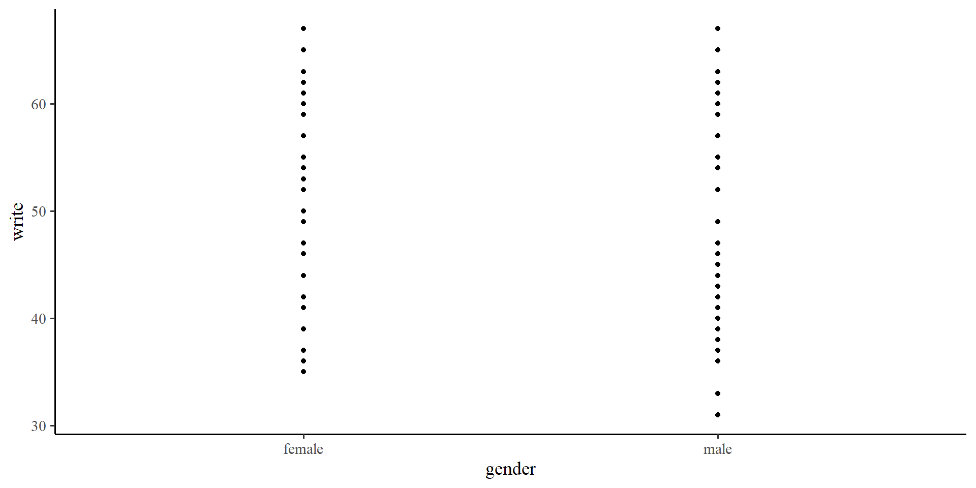
If we try to plot the write score on the \(y\)-axis and gender on the \(x\)-axis we can visualize observations in each group. But there are no “units” on the \(x\)-axis 🤔
However, it turns out that there are ways to trick regression into treating categorical variables as continuous!
But first, I would like to point something out…
Plot code
ggplot(hsb2, aes(x = gender, y = write)) +geom_point()
Intercept only Regression
You can use the lm() function with only one variable. Meaning, you can run a regression without any predictors (!?). for example, for the write variable:
car::S(lm(write ~1, data = hsb2))
Call: lm(formula = write ~ 1, data = hsb2)

Coefficients:
            Estimate Std. Error t value Pr(>|t|)
(Intercept)  52.7750     0.6702   78.74   <2e-16 ***
---
Signif. codes:  0 '***' 0.001 '**' 0.01 '*' 0.05 '.' 0.1 ' ' 1

Residual standard deviation: 9.479 on 199 degrees of freedom
    AIC     BIC
1470.19 1476.78
The intercept, \(52.78\) and the residual SD, \(9.47\). These values are the mean and SD of the write variable.
mean(hsb2$write)
[1] 52.775
sd(hsb2$write)
[1] 9.478586
This is consistent with the representation of regression shown in the appendix of Lab 2, Here \(Y \sim N(\mu = 52.78, \sigma = 9.47)\)
So regression with only the intercept estimates the mean and SD of \(Y\). But what now? Let’s look at the graphical representation of the intercept only model.
Intercept only model Visualized
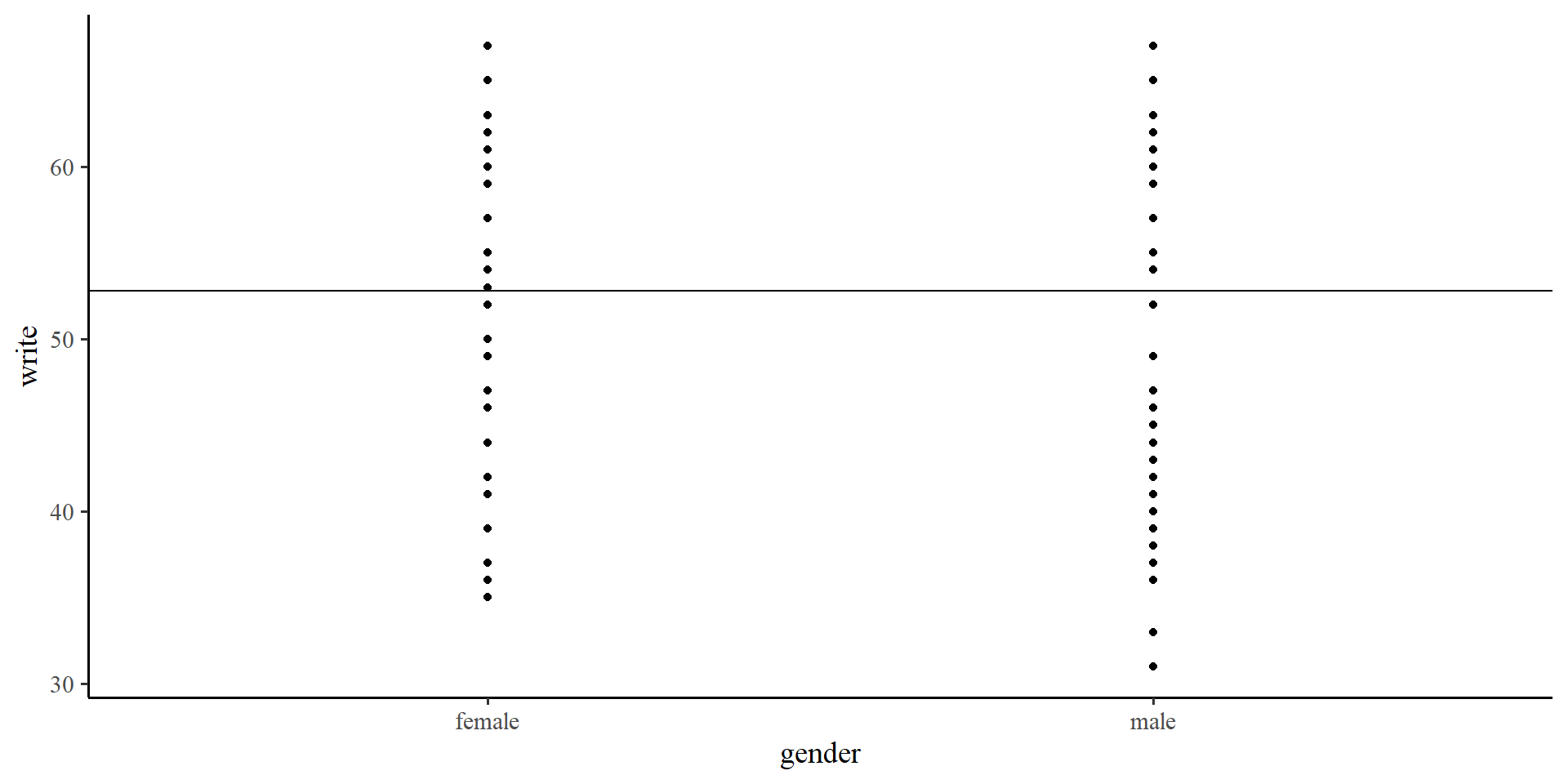
If we only use the intercept in out model, the “regression line” will be flat and intercept the \(y\)-axis at the mean of \(Y\).
…but wait a moment, we have two groups, female and male. How about we give each group their own intercept?
this simply implies that we believe that the mean of the \(Y\) variable, write, should differ based on gender.
Plot code
ggplot(hsb2, aes(x = gender, y = write)) +geom_point() +geom_hline(yintercept =mean(hsb2$write))
Group Means
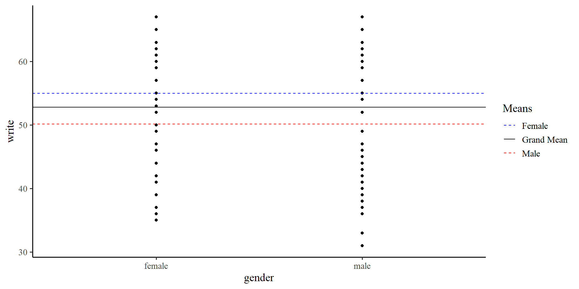
In the previous plot we were using the “grand mean” of write. If we use the two means instead…
We see that the means of the two groups are different.
# A tibble: 2 × 2
  gender Group_means
  <chr>        <dbl>
1 female        55.0
2 male          50.1
We can run a regression model that is the representation of the graph on the right
Plot code
mean_female <-mean(hsb2$write[hsb2$gender =="female"])mean_male <-mean(hsb2$write[hsb2$gender =="male"])ggplot(hsb2, aes(x = gender, y = write)) +geom_point() +geom_hline(aes(yintercept =mean(mean_female), color ="Female"), linetype ="dashed") +geom_hline(aes(yintercept =mean(mean_male), color ="Male"), linetype ="dashed") +geom_hline(aes(yintercept =mean(hsb2$write), color ="Grand Mean")) +scale_color_manual(values =c("Female"="blue", "Male"="red", "Grand Mean"="black")) +labs(color ="Means")
Coding Categorical Variables
We can code our categorical variables such that they are treated as continuous variables. Usually, we treat one group as “0”, and the other group as “1”. Let’s say that male is \(0\) and female is \(1\):
Remember that in regression, the intercept is expected mean value of \(Y\) when \(X = 0\), and the slope is the expected mean change in \(Y\) per unit increase in \(X\).
Then, since we coded \(0\) to represent male, the intercept is the mean of the male group in write score.
And, since we coded \(1\) to represent female, the slope is the difference in means between the male and female group in write score (\(50.12 + 4.87 = 54.99\)).
Mean differences? Sounds familiar?
We just tested whether male and female are significantly different in mean write score. This is what you should know as an independent-samples t-test (!).
t.test(hsb2$write ~ hsb2$gender,var.equal =TRUE)
    Two Sample t-test

data:  hsb2$write by hsb2$gender
t = 3.7341, df = 198, p-value = 0.0002463
alternative hypothesis: true difference in means between group female and group male is not equal to 0
95 percent confidence interval:
 2.298059 7.441835
sample estimates:
mean in group female   mean in group male
            54.99083             50.12088
You should see that t-values, degrees of freedom, and p-values are the same as those for the slope on the previous slide.
No Coincidences in Statistics
There are no coincidences in statistics. If two methods give some of the same results, they must be related in some way. When you see such patterns, ask yourself why two methods produce the same results. Once you answer that question, you will have gained tremendous insight.
t-tests don’t exist really. For some reason everyone decides to teach t-tests separately from regression, but they are simply a specific case of a regression.
The Values “Do not Matter”
Since gender is not really a continuous variable, so we can turn it into any numeric values and still run a regression. For example:
Call:
lm(formula = write ~ gender2, data = hsb2)

Residuals:
    Min      1Q  Median      3Q     Max
-19.991  -6.371   1.879   7.009  16.879

Coefficients:
             Estimate Std. Error t value Pr(>|t|)
(Intercept) 46.202531   1.876128  24.627  < 2e-16 ***
gender2     -0.027988   0.007495  -3.734 0.000246 ***
---
Signif. codes:  0 '***' 0.001 '**' 0.01 '*' 0.05 '.' 0.1 ' ' 1

Residual standard error: 9.185 on 198 degrees of freedom
Multiple R-squared:  0.06579,   Adjusted R-squared:  0.06107
F-statistic: 13.94 on 1 and 198 DF,  p-value: 0.0002463
The \(R^2\) is the exact same as the regression from 2 slides ago; whether we code male and female as \(0\) and \(1\) or \(-314\) and \(-140\) (some random numbers I chose), the models are equivalent. However, the values of the intercept and slope are now meaningless.
We can use this fact to our advantage! We can code our categorical variables in different ways to test hypotheses of mean differences between groups.
Note: We will go over some popular coding schemes, but you may devise your own depending on your hypotheses.
Dummy Coding
We have looked at the 2 groups case where we assigned \(0\) to one group and \(1\) to the other. However, what do we do when we have more than 2 groups?
The race variable, for example, has four groups:
unique(hsb2$race)
[1] "white" "african american" "hispanic" "asian"
We can’t assign different numbers to each group (e.g., \(0\), \(1\), \(2\), \(3\)) because then the variable will actually be treated as continuous.
Dummy coding is a coding scheme to represent a categorical variable with more than 2 categories.
In dummy coding, we use a series of \(0\)s and \(1\)s to define category membership. For example, we could say that:
c(1, 0, 0): African American
c(0, 1, 0): Hispanic
c(0, 0, 1): Asian
c(0, 0, 0): White
So, we will need 3 columns in our data that define the category membership of each one of our participants.
This is the most straightforward coding scheme. Let’s see what happens once we run a regression!
Creating Dummy coded Columns
The manual way of dummy coding variables in R involves creating separate columns. Here I show the dummy_columns() function from the fastDummies package.
The remove_most_frequent_dummy = TRUE argument turns the most frequent category, white in our case, into the c(0, 0, 0) group.
With this coding scheme, the c(0, 0, 0) group is going to be the reference group. It will be clear why once we run the regression and look at the results.
This function returns the same data, but with the added dummy coded columns. Here are the columns compared to the original variable:
Regression with Dummy coded Variables
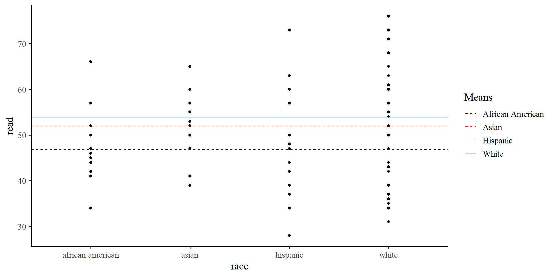
We want to test group difference in read scores across the race variable.
When all the dummy coded variables are \(0\), we get the intercept, so:
\(53.92 =\) the expected mean read score for white individuals.
\(-7.12 =\) the expected difference in mean read score for african american individuals compared to white individuals.
\(-2.02 =\) the expected difference in mean read score for asian individuals compared to white individuals.
\(-7.26 =\) the expected difference in mean read score for hispanic individuals compared to white individuals.
All the differences are with respect to the reference group, white. Further, the p-values of the slopes tell us whether the mean difference in read score between white and a specific group is significant!
# A tibble: 4 × 2
  race             `Group means`
  <chr>                    <dbl>
1 african american          46.8
2 asian                     51.9
3 hispanic                  46.7
4 white                     53.9
When calculating residuals, dummy coding tells the regression to switch to using the mean of a specific group when a member in that group is encountered.
Plot code
means <- hsb2 %>%group_by(race) %>%summarise(Group_means =mean(read)) %>% as.data.frameggplot(hsb2, aes(x = race, y = read)) +geom_point() +geom_hline(aes(yintercept = means[1,2], color ="African American"), linetype ="dashed") +geom_hline(aes(yintercept = means[2,2], color ="Asian"), linetype ="dashed") +geom_hline(aes(yintercept = means[3,2], color ="Hispanic")) +geom_hline(aes(yintercept = means[4,2], color ="White")) +scale_color_manual(values =c("African American"="blue", "Asian"="red", "Hispanic"="black","White"="cyan")) +labs(color ="Means")
So for asian individuals, the regression will use \(51.9\) to calculate residuals, for white individuals, the regression will use \(53.9\), and so on…
Multiple Mean differences? Also Familiar
We just ran what you may know as one-way ANOVA. If you remember from intro stats, the calculation for the sum or squares error (\(SSE\), the residuals) in ANOVAs involves this equation:
\[
\sum(X_{ij} - \bar{X}_j)^2,
\]
where \(X_{ij}\) is the observation of the \(i^{th}\) of individual in the \(j^{th}\) group, and \(\bar{X}_j\) is the mean of the \(j^{th}\) group. The \(\bar{X}_j\) part represents the mean that the residuals are calculated against changing for each group.
We can run a one-way ANOVA and see that we get the exact same \(F\)-value and degrees of freedom:
aov <-aov(read ~factor(race), data = hsb2)summary(aov)
              Df Sum Sq Mean Sq F value   Pr(>F)
factor(race)   3   1750   583.3   5.964 0.000654 ***
Residuals    196  19170    97.8
---
Signif. codes:  0 '***' 0.001 '**' 0.01 '*' 0.05 '.' 0.1 ' ' 1
From the regression summary:
summary(reg_race)$fstatistic
     value      numdf      dendf
  5.963662   3.000000 196.000000
Factor Variables in R
Coding variables manually takes some effort on the user’s end. We can use factor variables to make the process smoother.
we use the factor() function to turn any variable into a factor. Let’s turn the race variable into a factor:
Call:
lm(formula = read ~ race, data = hsb2)
Residuals:
Min 1Q Median 3Q Max
-22.924 -6.924 0.200 8.337 26.333
Coefficients:
Estimate Std. Error t value Pr(>|t|)
(Intercept) 53.9241 0.8213 65.658 < 2e-16 ***
raceAA -7.1241 2.3590 -3.020 0.00286 **
raceA -2.0150 3.0929 -0.652 0.51548
raceH -7.2575 2.1794 -3.330 0.00104 **
---
Signif. codes: 0 '***' 0.001 '**' 0.01 '*' 0.05 '.' 0.1 ' ' 1
Residual standard error: 9.89 on 196 degrees of freedom
Multiple R-squared: 0.08365, Adjusted R-squared: 0.06962
F-statistic: 5.964 on 3 and 196 DF, p-value: 0.0006539
This is the exact regression output from some slides ago, but we did not have to create all the dummy coded columns manually 😀
If you are using R, I recommend using factor variables rather than manually creating dummy coded variables.
Factor Variables are R specific
Every programming language has some common variable types (e.g., double, integer, character,…), but, as far as I can tell, factor variables are unique to R. The R programming language was created with statistics in mind. The fact that factor variables automatically dummy code categorical variables is a reflection of that.
Other coding schemes
So far we coded our race variable such that all the groups are compared to the white group. We can test different hypotheses if we change our coding scheme. Thanks to the way factor variables work, there is an elegant way of changing coding schemes!
The contrast matrix that defines the coding scheme is a property stored in every factor variable.
contrasts(hsb2$race)
   AA A H
W   0 0 0
AA  1 0 0
A   0 1 0
H   0 0 1
We can directly edit contrast matrix of a factor variable to change coding schemes. R also provides a series of functions that generate commonly used contrast matrices. For example:
# `4` stands for number of groupscontr.sum(4)
  [,1] [,2] [,3]
1    1    0    0
2    0    1    0
3    0    0    1
4   -1   -1   -1
To edit the default contrast matrix inside a factor we use the assignment operator:
contrasts(hsb2$race) <-contr.sum(4)# the contrast matrix has been updatedcontrasts(hsb2$race)
   [,1] [,2] [,3]
W     1    0    0
AA    0    1    0
A     0    0    1
H    -1   -1   -1
This type of coding scheme is known as unweighted effects coding. The unweighted part comes from the fact that the grand mean is calculated by assuming that every groups has the same sample size.
Call:
lm(formula = read ~ race, data = hsb2)

Residuals:
    Min      1Q  Median      3Q     Max
-22.924  -6.924   0.200   8.337  26.333

Coefficients:
            Estimate Std. Error t value Pr(>|t|)
(Intercept)   49.825      1.076  46.297  < 2e-16 ***
race1          4.099      1.223   3.352 0.000963 ***
race2         -3.025      1.898  -1.594 0.112644
race3          2.084      2.367   0.880 0.379722
---
Signif. codes:  0 '***' 0.001 '**' 0.01 '*' 0.05 '.' 0.1 ' ' 1

Residual standard error: 9.89 on 196 degrees of freedom
Multiple R-squared:  0.08365,   Adjusted R-squared:  0.06962
F-statistic: 5.964 on 3 and 196 DF,  p-value: 0.0006539
The intercept, \(49.82\), is the unweighted grand mean (it’s the mean of the group means).
Given the way we coded our factor, the slopes test whether either W, AA, or A individuals are significantly different in mean read score from the unweighted grand mean.
The only significantly different group is the W group, which was coded as c(1, 0, 0). We can get the mean by plugging the values into the regression:
You can do the same for all the the other rows of the matrix on the previous slide and you will see that you will get the means of every group.
Also note that in this type of contrast, the row with c(-1,-1,-1), H in our case, is always “left out”, as we don’t test any hypotheses about it directly.
Weighted Effects Coding
The contr.sum() function creates contrasts assuming that all groups have the same number of participants. This is not true in out case:
This is our current contrast matrix for the race variable.
contrasts(hsb2$race)
   [,1] [,2] [,3]
W     1    0    0
AA    0    1    0
A     0    0    1
H    -1   -1   -1
The groups definitely do not have the same sample size.
table(hsb2$race)
  W  AA   A   H
145  20  11  24
if \(N_H\) is the sample size for the H group, then we achieve weighted effects coding by substituting the last row with \(\mathrm{c}(-\frac{N_W}{N_H}, -\frac{N_{AA}}{N_H}, -\frac{N_A}{N_H})\)
we can edit the last row of the contrast matrix of race directly:
Call:
lm(formula = read ~ race, data = hsb2)

Residuals:
    Min      1Q  Median      3Q     Max
-22.924  -6.924   0.200   8.337  26.333

Coefficients:
            Estimate Std. Error t value Pr(>|t|)
(Intercept)  52.2300     0.6993  74.689  < 2e-16 ***
race1         1.6941     0.4307   3.934 0.000116 ***
race2        -5.4300     2.0979  -2.588 0.010368 *
race3        -0.3209     2.8987  -0.111 0.911960
---
Signif. codes:  0 '***' 0.001 '**' 0.01 '*' 0.05 '.' 0.1 ' ' 1

Residual standard error: 9.89 on 196 degrees of freedom
Multiple R-squared:  0.08365,   Adjusted R-squared:  0.06962
F-statistic: 5.964 on 3 and 196 DF,  p-value: 0.0006539
Now the intercept, \(52.32\), which is the grand mean of read score!
mean(hsb2$read)
[1] 52.23
Thus, the coefficients represent the the deviation of the W, AA, and A group in read score compared to the average read score for the whole sample.
The W group is \(1.69\) points higher in read score points compared to the sample average. (significant)
The AA group is \(5.43\) points lower in read score points compared to the sample average. (significant)
The A group is \(0.32\) points lower in read score points compared to the sample average. (not significant)
On the previous slide, we just changed the last row of the contrast matrix. You can also change the contrast matrix in its entirety if your hypotheses involve different contrasts. You need to know how to set up the contrasts matrix such that the coefficients test the hypotheses you want. see Here a detailed explanation of contrasts.
Why all These Contrasts? 😕 A summary
All of this contrast matrix talk may seem very confusing. You have the field of experimental psychology to thank for it 😅 I don’t run experiments myself, so I don’t think much about all of this.
Jokes aside, contrasts are used to test hypotheses. You can test any type of mean comparison hypothesis by specifying the appropriate contrast.
Why are we “allowed” to mess with regression coefficients in this way? As previously mentioned, categorical variables have no meaningful numerical scale (e.g., we don’t say “pasta 🍝 is greater than pizza 🍕”).
However, we can assign some numerical scale to categorical variables such that the regression coefficients are “forced” to test the hypotheses we are interested in.
Do you need contrast matrices when testing hypotheses? Nah 🤷 In practice, you can just compare group means one by one (assuming you apply some Type I error rate correction if you are using p-values). However, contrast matrices are an elegant way of testing multiple hypotheses at once.
Personal opinion: Experimental psychologists really like their elegant designs, maybe a bit too much. It is my sense that contrast matrices are mostly a product of computational limitations of the past. These days, especially if you do Bayesian statistics, contrast do not have many uses (at least for mean comparisons).